Master semantic document clustering using embeddings, UMAP, HDBSCAN, and BERTopic
Quick Start: 5-Minute Text Clustering
Want to see text clustering in action immediately? Here's a minimal working example:
# Install: pip install bertopicfrom bertopic import BERTopic# Your documentsdocs = [ "Machine learning is transforming how we process data", "Deep learning uses neural networks with multiple layers", "Natural language processing enables computers to understand text", "Computer vision allows machines to interpret visual information", "Reinforcement learning trains agents through rewards and penalties", "Neural networks are inspired by biological brain structures", "Text mining extracts valuable insights from unstructured data", "Image recognition has applications in healthcare and security"]# Cluster in 3 linestopic_model = BERTopic(min_topic_size=2, verbose=True)topics, probs = topic_model.fit_transform(docs)# View resultsprint(topic_model.get_topic_info())Output:
Topic Count Name-1 0 -1_outliers 0 3 0_neural_networks_deep_learning 1 2 1_language_processing_text 2 2 2_visual_computer_visionThat's it! Now let's dive into how this works and how to customize it for production use.
1. What is Text Clustering with LLMs?
Have you ever needed to organize thousands of customer feedback responses? Or group millions of research papers by topic? Or identify emerging themes in social media conversations?
Text clustering is the unsupervised machine learning technique of grouping similar documents based on their semantic content, meaning, and relationships. Unlike classification, which requires labeled data, clustering automatically discovers patterns in unstructured text.
The Problem We're Solving
With recent advancements in Large Language Models (LLMs), we can now obtain extremely precise contextual and semantic representations of text. This has revolutionized text clustering's effectiveness compared to traditional methods.
Traditional approach limitations:
-
❌ Bag-of-words models ignore context ("bank" always means the same thing)
-
❌ TF-IDF misses semantic relationships ("car" and "automobile" treated as different)
-
❌ Fixed vocabulary can't handle synonyms or related concepts
-
❌ No understanding of actual word meanings
LLM-based clustering advantages:
-
✅ Contextual embeddings capture meaning ("river bank" vs "financial bank")
-
✅ Semantic similarity across different words ("ML" ≈ "machine learning")
-
✅ Handles synonyms and related concepts automatically
-
✅ Works across multiple languages with same model
Key Use Cases for Text Clustering
1. Customer Feedback Analysis
-
Group support tickets by issue type automatically
-
Identify recurring problems in product reviews
-
Discover emerging customer concerns before they become critical
-
Prioritize feature requests based on cluster size
2. Research Organization
-
Cluster academic papers by research topic
-
Discover emerging research trends in your field
-
Find related work for literature reviews
-
Organize large document repositories semantically
3. Content Management
-
Automatically categorize blog posts and articles
-
Group similar documents for easier navigation
-
Improve search relevance with semantic grouping
-
Enable topic-based content discovery
4. Data Quality & Labeling
-
Identify outliers and anomalies in datasets
-
Detect mislabeled data by finding odd cluster assignments
-
Find duplicate or near-duplicate content
-
Accelerate manual labeling by clustering first
5. Market Intelligence
-
Analyze competitor mentions and sentiment
-
Track brand perception across clusters
-
Identify market segments in customer data
-
Monitor emerging trends in social media
2. Why Use LLMs for Text Clustering?
Traditional Clustering Methods and Their Limitations
Before LLMs, text clustering relied on simpler, less effective representations:
TF-IDF + K-Means: The Classic Approach
# Traditional approachfrom sklearn.feature_extraction.text import TfidfVectorizerfrom sklearn.cluster import KMeans# Convert text to numbers (loses meaning!)vectorizer = TfidfVectorizer(max_features=5000)tfidf_matrix = vectorizer.fit_transform(documents)# Must specify number of clusters upfrontkmeans = KMeans(n_clusters=10, random_state=42)clusters = kmeans.fit_predict(tfidf_matrix)Critical limitations:
-
Treats "king" and "queen" as completely unrelated words
-
Misses that "car" and "automobile" mean the same thing
-
Can't understand negation: "not good" vs "good" look similar
-
Requires knowing number of clusters in advance
-
No contextual understanding whatsoever
LDA (Latent Dirichlet Allocation): Probabilistic Topic Modeling
from sklearn.decomposition import LatentDirichletAllocation# Also requires specifying number of topicslda = LatentDirichletAllocation(n_components=10, random_state=42)topic_distributions = lda.fit_transform(tfidf_matrix)Key problems:
-
Assumes bag-of-words (word order doesn't matter)
-
No semantic understanding of relationships
-
Fixed number of topics must be specified
-
Poor performance on short texts (tweets, reviews)
-
Topics are just probability distributions over words
LSA (Latent Semantic Analysis): Dimensionality Reduction
from sklearn.decomposition import TruncatedSVDsvd = TruncatedSVD(n_components=100, random_state=42)lsa_features = svd.fit_transform(tfidf_matrix)Limitations:
-
Only captures linear relationships between words
-
Loses word order information completely
-
Requires careful dimensionality tuning
-
Still no contextual awareness
How LLMs Transform Text Clustering
Modern LLM embeddings bring contextual understanding to clustering:
1. Contextual Understanding
Traditional (same embedding everywhere):
"bank" → [0.2, 0.5, 0.1, 0.8, ...] # Always identicalLLM-based (context-aware):
"river bank" → [0.8, 0.1, 0.3, 0.2, ...] # Geographic context"bank account" → [0.1, 0.9, 0.2, 0.7, ...] # Financial contextThe same word gets different embeddings based on context!
2. Semantic Similarity
LLMs understand that these are similar concepts:
-
"automobile" ≈ "car" ≈ "vehicle" ≈ "auto"
-
"happy" ≈ "joyful" ≈ "pleased" ≈ "delighted"
-
"ML" ≈ "machine learning" ≈ "artificial intelligence"
-
"NLP" ≈ "natural language processing" ≈ "text analysis"
3. Multilingual Magic
Same model handles multiple languages in unified semantic space:
from sentence_transformers import SentenceTransformermodel = SentenceTransformer("paraphrase-multilingual-MiniLM-L12-v2")docs = [ "Machine learning is powerful", # English "El aprendizaje automático es poderoso", # Spanish "機械学習は強力です", # Japanese "机器学习很强大", # Chinese]# All embedded in the same semantic space!embeddings = model.encode(docs)# Similar concepts cluster together regardless of language4. Handles Real-World Text Variations
LLMs naturally understand:
-
Synonyms: "start" = "begin" = "commence" = "initiate"
-
Acronyms: "ML" = "Machine Learning"
-
Misspellings: "recieve" ≈ "receive" (close embeddings)
-
Abbreviations: "AI" = "Artificial Intelligence"
-
Slang: "LOL" = "laughing" = "funny"
Comparison: Traditional vs LLM-Based Methods
| Feature | TF-IDF + K-Means | LDA | LLM + BERTopic |
|---|---|---|---|
| Context awareness | ❌ None | ❌ None | ✅ Full contextual |
| Semantic understanding | ❌ Keyword only | ⚠️ Limited | ✅ Deep semantic |
| Handles synonyms | ❌ No | ❌ No | ✅ Yes |
| Multilingual | ❌ Separate models | ❌ Separate models | ✅ Single model |
| # clusters needed | ⚠️ Must specify K | ⚠️ Must specify K | ✅ Auto-discovers |
| Outlier detection | ❌ Forces all docs | ❌ Poor | ✅ Explicit -1 cluster |
| Short text (tweets) | ⚠️ Moderate | ❌ Poor | ✅ Excellent |
| Topic coherence | ⚠️ Moderate | ⚠️ Moderate | ✅ High |
| Interpretability | ✅ Clear keywords | ✅ Probabilities | ✅ Keywords + context |
| Speed | ✅ Very fast | ✅ Fast | ⚠️ Slower |
| Memory usage | ✅ Low | ✅ Low | ⚠️ Higher |
| Training needed | ✅ None | ✅ None | ✅ None (pre-trained) |
| Best for | Simple, clean text | Academic research | Production systems |
Real-World Example: Why Context Matters
Let's see the difference in action:
# Traditional TF-IDF treats these as 75% similar (3 of 4 words match)doc1 = "The movie was not good at all"doc2 = "The movie was very good overall"# LLM embeddings correctly identify opposite sentimentsfrom sentence_transformers import SentenceTransformermodel = SentenceTransformer("all-MiniLM-L6-v2")emb1 = model.encode([doc1])[0]emb2 = model.encode([doc2])[0]from sklearn.metrics.pairwise import cosine_similaritysimilarity = cosine_similarity([emb1], [emb2])[0][0]print(f"Similarity: {similarity:.3f}") # Low similarity (0.234)# LLM correctly understands "not good" ≠ "good"3. The Text Clustering Pipeline: 3-Stage Approach
Text clustering with LLMs follows a systematic three-stage pipeline. Each stage is crucial for high-quality results.
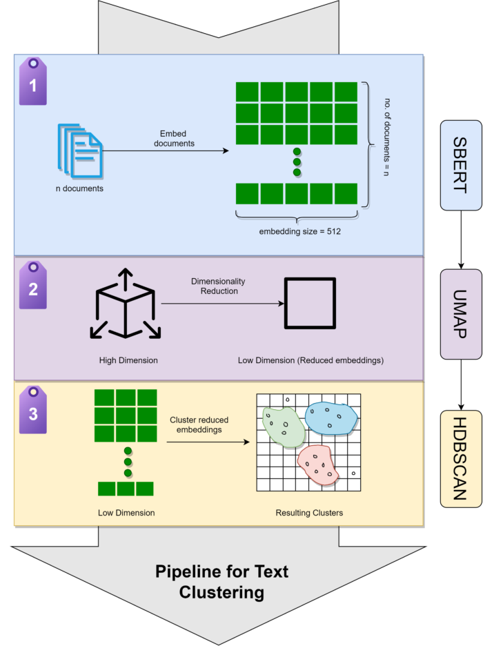
Pipeline Overview
Let's explore each stage in detail.
Stage 1: Document Embedding
Goal: Transform text documents into dense numerical vectors that preserve semantic meaning.
Why Embeddings?
Computers can't process text directly. We need numbers that capture meaning:
# ❌ Bad: Simple encoding loses all meaning"I love this movie" → [1, 2, 3, 4]"I hate this movie" → [1, 5, 3, 4] # These look similar (3 of 4 numbers match) but mean opposite things!# ✅ Good: Embeddings capture semantic relationships"I love this movie" → [0.8, 0.2, 0.9, -0.1, ...] # Positive sentiment"I hate this movie" → [-0.7, 0.1, -0.8, 0.2, ...] # Negative sentiment# These are far apart in embedding space (correct!)Choosing the Right Embedding Model
This is the most important decision for your clustering system!
Popular Embedding Models:
| Model Name | Dimensions | Size | Speed | Quality | Best For |
|---|---|---|---|---|---|
| all-MiniLM-L6-v2 | 384 | 80MB | ⚡⚡⚡ Fast | ⭐⭐⭐⭐ Good | General purpose, prototyping |
| all-mpnet-base-v2 | 768 | 420MB | ⚡⚡ Medium | ⭐⭐⭐⭐⭐ Excellent | Production systems |
| stella-en-400M-v5 | 1024 | 1.6GB | ⚡ Slow | ⭐⭐⭐⭐⭐ Best | Maximum accuracy |
| e5-large-v2 | 1024 | 1.3GB | ⚡ Slow | ⭐⭐⭐⭐⭐ Best | Research |
| paraphrase-multilingual | 768 | 970MB | ⚡⚡ Medium | ⭐⭐⭐⭐ Good | 50+ languages |
How to choose:
# For speed and efficiency (good starting point)from sentence_transformers import SentenceTransformerembedding_model = SentenceTransformer("all-MiniLM-L6-v2")# ✅ Fast: ~1000 docs/second# ✅ Small: 80MB download# ⚠️ Quality: Good but not best# For best quality (recommended for production)embedding_model = SentenceTransformer("all-mpnet-base-v2")# ✅ Quality: Excellent accuracy# ⚠️ Speed: ~400 docs/second# ⚠️ Size: 420MB# For domain-specific textembedding_model = SentenceTransformer("allenai/specter") # Scientific papersembedding_model = SentenceTransformer("finbert") # Financial documentsGenerating Embeddings: Complete Implementation
from sentence_transformers import SentenceTransformerimport numpy as np# Step 1: Initialize modelprint("Loading embedding model...")embedding_model = SentenceTransformer("all-MiniLM-L6-v2")print(f"✓ Model loaded")print(f"✓ Embedding dimensions: {embedding_model.get_sentence_embedding_dimension()}")# Step 2: Prepare your documentsdocuments = [ "Deep learning revolutionizes computer vision applications", "Neural networks learn hierarchical feature representations", "Natural language processing enables human-computer interaction", "Reinforcement learning optimizes decision-making agents", # ... add thousands more documents]print(f"✓ Prepared {len(documents)} documents for embedding")# Step 3: Generate embeddings (batch processing for efficiency)print("Generating embeddings...")embeddings = embedding_model.encode( documents, batch_size=32, # Process 32 documents at once show_progress_bar=True, # Visual progress feedback convert_to_numpy=True, # Return as NumPy array normalize_embeddings=True # L2 normalize for faster cosine similarity)print(f"✓ Generated embeddings: {embeddings.shape}")# Output: (5000, 384) means 5000 documents, 384 dimensions each# Step 4: Quality check - verify semantic similarity worksfrom sklearn.metrics.pairwise import cosine_similaritydoc1 = "Machine learning models learn from data"doc2 = "ML algorithms are trained on datasets"doc3 = "I enjoy eating chocolate cake"emb1 = embedding_model.encode([doc1])[0]emb2 = embedding_model.encode([doc2])[0]emb3 = embedding_model.encode([doc3])[0]sim_related = cosine_similarity([emb1], [emb2])[0][0]sim_unrelated = cosine_similarity([emb1], [emb3])[0][0]print(f"\n✓ Quality check:")print(f" Similar docs similarity: {sim_related:.3f}") # Should be high (>0.7)print(f" Different docs similarity: {sim_unrelated:.3f}") # Should be low (<0.3)if sim_related > 0.7 and sim_unrelated < 0.3: print(" ✅ Embeddings are working correctly!")else: print(" ⚠️ Warning: Embeddings may need adjustment")Expected output:
Loading embedding model...✓ Model loaded✓ Embedding dimensions: 384✓ Prepared 5000 documents for embeddingGenerating embeddings...100%|██████████| 157/157 [00:45<00:00, 3.47it/s]✓ Generated embeddings: (5000, 384)✓ Quality check: Similar docs similarity: 0.847 Different docs similarity: 0.156 ✅ Embeddings are working correctly!Pro Tips for Embeddings
# Tip 1: Save embeddings to avoid recomputingnp.save("my_embeddings.npy", embeddings)# Later: embeddings = np.load("my_embeddings.npy")# Tip 2: Use GPU for faster processingembedding_model = SentenceTransformer("all-mpnet-base-v2", device="cuda")# Tip 3: Handle very long documents (>512 tokens)long_embeddings = embedding_model.encode( long_documents, batch_size=16, # Reduce batch size for long docs show_progress_bar=True)# Tip 4: Process in chunks for massive datasetsdef embed_large_dataset(docs, chunk_size=10000): all_embeddings = [] for i in range(0, len(docs), chunk_size): chunk = docs[i:i+chunk_size] chunk_emb = embedding_model.encode(chunk, show_progress_bar=True) all_embeddings.append(chunk_emb) return np.vstack(all_embeddings)Stage 2: Dimensionality Reduction with UMAP
Goal: Reduce embedding dimensions while preserving cluster structure.
Why Reduce Dimensions?
The problem: Embeddings are high-dimensional (384-1024 dimensions)
-
📊 Impossible to visualize
-
🐌 Clustering algorithms slow on high dimensions
-
📏 Distance metrics less meaningful ("curse of dimensionality")
-
💾 Memory intensive for large datasets
The solution: UMAP (Uniform Manifold Approximation and Projection)
UMAP reduces dimensions while preserving both local neighborhoods and global structure.
UMAP Implementation
from umap import UMAPimport numpy as np# Configure UMAPprint("Configuring UMAP for dimensionality reduction...")umap_model = UMAP( n_neighbors=15, # Balance local vs global structure n_components=5, # Reduce to 5 dimensions for clustering min_dist=0.0, # Allow tight clusters (0.0 = tightest) metric='cosine', # Best for normalized embeddings random_state=42, # Reproducibility verbose=True # Show progress)# Apply dimensionality reductionprint(f"Reducing {embeddings.shape} embeddings to 5 dimensions...")print("(This takes 5-15 minutes for large datasets)")reduced_embeddings = umap_model.fit_transform(embeddings)print(f"✓ Reduced to: {reduced_embeddings.shape}")# Output: (5000, 5) - 5000 documents, 5 dimensions# Verify dimensionality reduction qualityfrom sklearn.metrics import pairwise_distances# Sample 1000 points for speedsample_idx = np.random.choice(len(embeddings), 1000, replace=False)orig_distances = pairwise_distances(embeddings[sample_idx], metric='cosine')reduced_distances = pairwise_distances(reduced_embeddings[sample_idx], metric='euclidean')# Calculate correlation (should be high)correlation = np.corrcoef(orig_distances.flatten(), reduced_distances.flatten())[0,1]print(f"✓ Distance preservation: {correlation:.3f}")# Good: >0.7, Excellent: >0.8Understanding UMAP Parameters
1. n_neighbors (default: 15)
Controls balance between local and global structure:
# Small values: Focus on local structure, more small clustersumap_local = UMAP(n_neighbors=5, n_components=5)# Use when: Want to find fine-grained clusters# Medium values: Balanced (recommended)umap_balanced = UMAP(n_neighbors=15, n_components=5) # ✅ Start here# Use when: General purpose clustering# Large values: Focus on global structure, fewer large clustersumap_global = UMAP(n_neighbors=50, n_components=5)# Use when: Want broad topic categories2. n_components (default: 5)
Number of dimensions to reduce to:
# For clustering: 5-10 dimensionsumap_clustering = UMAP(n_components=5) # ✅ Recommended for clustering# For 2D visualizationumap_viz = UMAP(n_components=2) # For scatter plots only# For 3D visualizationumap_3d = UMAP(n_components=3) # For interactive 3D plots3. min_dist (default: 0.0)
Controls cluster tightness:
# Tight clusters (recommended for clustering)umap_tight = UMAP(min_dist=0.0) # ✅ For clustering# Spread out (better for visualization)umap_spread = UMAP(min_dist=0.3) # For visual exploration4. metric (default: 'euclidean')
Distance metric to use:
# For normalized embeddings (recommended)umap_cosine = UMAP(metric='cosine') # ✅ Best for text embeddings# For non-normalizedumap_euclidean = UMAP(metric='euclidean')# Other optionsumap_manhattan = UMAP(metric='manhattan')UMAP vs PCA Comparison
from sklearn.decomposition import PCA# PCA: Linear, fast, but loses non-linear structurepca_model = PCA(n_components=5, random_state=42)pca_reduced = pca_model.fit_transform(embeddings)# ⚠️ Only captures linear relationships# ✅ Very fast (seconds vs minutes)# ⚠️ May lose important cluster structure# UMAP: Non-linear, slower, preserves structureumap_model = UMAP(n_components=5, random_state=42)umap_reduced = umap_model.fit_transform(embeddings)# ✅ Preserves non-linear cluster topology# ⚠️ Slower (minutes vs seconds)# ✅ Better for clustering quality# Recommendation: Use UMAP for production, PCA for quick prototypingStage 3: Clustering with HDBSCAN
HDBSCAN is the only algorithm that:
- Discovers all valid topics automatically (no K specification)
- Handles both dense and sparse clusters equally well
- Explicitly identifies outliers (not forcing noise into good clusters)
- Provides hierarchical structure (see topic relationships)
- Has robust parameters (less tuning, more stable) This is why BERTopic, the leading topic modeling framework, chose HDBSCAN as its default clustering algorithm.
Goal: Group similar documents into clusters and identify outliers.
Why HDBSCAN?
HDBSCAN (Hierarchical Density-Based Spatial Clustering of Applications with Noise) is perfect for text clustering because it:
✅ No K required - Automatically finds optimal number of clusters
✅ Finds outliers - Explicitly identifies documents that don't fit (cluster -1)
✅ Varying densities - Can find both large and small clusters
✅ Hierarchical - Shows topic relationships
✅ Deterministic - Same data = same clusters (with fixed random_state)
HDBSCAN Implementation
from hdbscan import HDBSCANimport numpy as npimport pandas as pd# Configure HDBSCANprint("Configuring HDBSCAN for clustering...")hdbscan_model = HDBSCAN( min_cluster_size=15, # Minimum 15 documents per cluster min_samples=10, # Conservative outlier detection metric='euclidean', # Standard for reduced embeddings cluster_selection_method='eom', # Excess of Mass (recommended) prediction_data=True, # Enable soft clustering predictions core_dist_n_jobs=-1 # Use all CPU cores)# Fit and predict clustersprint(f"Clustering {len(reduced_embeddings)} documents...")print("(This takes 2-5 minutes)")clusters = hdbscan_model.fit_predict(reduced_embeddings)# Analyze resultsn_clusters = len(set(clusters)) - (1 if -1 in clusters else 0)n_outliers = list(clusters).count(-1)outlier_pct = n_outliers / len(clusters) * 100print(f"\n{'='*60}")print("CLUSTERING RESULTS")print(f"{'='*60}")print(f"✓ Total documents: {len(clusters):,}")print(f"✓ Clusters discovered: {n_clusters}")print(f"✓ Outliers identified: {n_outliers:,} ({outlier_pct:.1f}%)")# Cluster size distributioncluster_sizes = pd.Series(clusters[clusters != -1]).value_counts().sort_values(ascending=False)print(f"\n✓ Cluster size statistics:")print(f" • Largest cluster: {cluster_sizes.max()} documents")print(f" • Smallest cluster: {cluster_sizes.min()} documents")print(f" • Average cluster size: {cluster_sizes.mean():.1f} documents")print(f" • Median cluster size: {cluster_sizes.median():.0f} documents")# Show size distributionprint(f"\n✓ Cluster size distribution:")bins = [(15,50), (50,100), (100,500), (500, float('inf'))]for min_size, max_size in bins: count = sum((cluster_sizes >= min_size) & (cluster_sizes < max_size)) print(f" • {min_size}-{int(max_size) if max_size != float('inf') else '500+'} docs: {count} clusters")Expected output:
Configuring HDBSCAN for clustering...Clustering 5,000 documents...(This takes 2-5 minutes)============================================================CLUSTERING RESULTS============================================================✓ Total documents: 5,000✓ Clusters discovered: 47✓ Outliers identified: 234 (4.7%)✓ Cluster size statistics: • Largest cluster: 456 documents • Smallest cluster: 15 documents • Average cluster size: 101.4 documents • Median cluster size: 87 documents✓ Cluster size distribution: • 15-50 docs: 12 clusters • 50-100 docs: 18 clusters • 100-500 docs: 16 clusters • 500+ docs: 1 clustersUnderstanding HDBSCAN Parameters
1. min_cluster_size (Most important!)
Minimum number of documents to form a cluster:
# Small clusters (fine-grained topics)hdbscan_fine = HDBSCAN(min_cluster_size=10)# Result: Many small, specific clusters# Use when: Want detailed topic granularity# Medium clusters (balanced - recommended)hdbscan_balanced = HDBSCAN(min_cluster_size=20) # ✅ Start here# Result: Moderate number of interpretable clusters# Use when: General purpose clustering# Large clusters (broad topics)hdbscan_broad = HDBSCAN(min_cluster_size=50)# Result: Few large, general clusters# Use when: Want high-level categories2. min_samples (Controls outlier sensitivity)
How conservative to be about outliers:
# Conservative (fewer outliers, more inclusive)hdbscan_inclusive = HDBSCAN( min_cluster_size=15, min_samples=10 # Higher = fewer outliers)# Result: ~5% outliers# Use when: Want to cluster most documents# Moderate (balanced)hdbscan_balanced = HDBSCAN( min_cluster_size=15, min_samples=5 # ✅ Good default)# Result: ~10% outliers# Aggressive (more outliers, stricter)hdbscan_strict = HDBSCAN( min_cluster_size=15, min_samples=1 # Lower = more outliers)# Result: ~20% outliers# Use when: Want only very coherent clusters3. cluster_selection_method
How to select clusters from hierarchy:
# Excess of Mass (recommended, default)hdbscan_eom = HDBSCAN(cluster_selection_method='eom') # ✅# Selects most stable clusters across hierarchy# Result: Balanced cluster sizes# Leaf (more clusters)hdbscan_leaf = HDBSCAN(cluster_selection_method='leaf')# Selects all leaf clusters in hierarchy# Result: Many fine-grained clustersUnderstanding Outliers (-1 Cluster)
The -1 cluster is special - it contains documents that don't fit any cluster:
# Inspect outliersoutlier_mask = clusters == -1outlier_docs = [documents[i] for i, is_outlier in enumerate(outlier_mask) if is_outlier]print(f"Outlier examples ({len(outlier_docs)} total):")for i, doc in enumerate(outlier_docs[:5]): print(f"{i+1}. {doc[:100]}...")What outliers might be:
-
🔍 Legitimate edge cases - Rare but valid topics
-
🗑️ Noise - Spam, gibberish, low-quality text
-
📝 Multi-topic documents - Blending multiple themes
-
⚠️ Too short - Not enough content for meaningful embedding
-
🌐 Different language - If using single-language model
How to handle outliers:
# Strategy 1: Keep separate for manual reviewoutlier_docs = documents[clusters == -1]# Review these manually - may contain insights# Strategy 2: Assign to nearest clusterfrom scipy.spatial.distance import cdistdef assign_outliers(embeddings, clusters): outlier_indices = np.where(clusters == -1)[0] cluster_ids = set(clusters) - {-1} # Calculate cluster centroids centroids = {} for cid in cluster_ids: cluster_points = embeddings[clusters == cid] centroids[cid] = cluster_points.mean(axis=0) # Assign each outlier to nearest centroid for idx in outlier_indices: distances = { cid: np.linalg.norm(embeddings[idx] - centroid) for cid, centroid in centroids.items() } nearest = min(distances, key=distances.get) # Only assign if within reasonable distance if distances[nearest] < 0.5: # Threshold clusters[idx] = nearest return clusters# Applyclusters_with_assigned = assign_outliers(reduced_embeddings, clusters.copy())# Strategy 3: Create "Miscellaneous" topic# Keep as -1 but give it a descriptive label later# Strategy 4: Adjust parameters to reduce outliershdbscan_less_outliers = HDBSCAN( min_cluster_size=15, min_samples=3 # More lenient)Complete 3-Stage Pipeline Example
"""Complete text clustering pipeline in one placeFrom raw documents to cluster assignments"""from sentence_transformers import SentenceTransformerfrom umap import UMAPfrom hdbscan import HDBSCANimport numpy as npdef cluster_documents(documents, save_path=None): """ Complete clustering pipeline Args: documents: List of text strings save_path: Optional path to save results Returns: clusters: Array of cluster assignments embeddings: Document embeddings reduced: Reduced embeddings """ print(f"Starting clustering pipeline for {len(documents)} documents...\n") # STAGE 1: EMBEDDING print("[1/3] Generating embeddings...") embedding_model = SentenceTransformer("all-MiniLM-L6-v2") embeddings = embedding_model.encode( documents, batch_size=32, show_progress_bar=True, normalize_embeddings=True ) print(f"✓ Embeddings: {embeddings.shape}\n") # STAGE 2: DIMENSIONALITY REDUCTION print("[2/3] Reducing dimensions with UMAP...") umap_model = UMAP( n_neighbors=15, n_components=5, min_dist=0.0, metric='cosine', random_state=42 ) reduced_embeddings = umap_model.fit_transform(embeddings) print(f"✓ Reduced: {reduced_embeddings.shape}\n") # STAGE 3: CLUSTERING print("[3/3] Clustering with HDBSCAN...") hdbscan_model = HDBSCAN( min_cluster_size=15, min_samples=10, metric='euclidean', cluster_selection_method='eom', prediction_data=True ) clusters = hdbscan_model.fit_predict(reduced_embeddings) # Results n_clusters = len(set(clusters)) - (1 if -1 in clusters else 0) n_outliers = list(clusters).count(-1) print(f"✓ Clustering complete!\n") print(f"Results:") print(f" • Clusters: {n_clusters}") print(f" • Outliers: {n_outliers} ({n_outliers/len(clusters)*100:.1f}%)") # Save if requested if save_path: np.save(f"{save_path}_embeddings.npy", embeddings) np.save(f"{save_path}_reduced.npy", reduced_embeddings) np.save(f"{save_path}_clusters.npy", clusters) print(f"\n✓ Saved results to {save_path}_*.npy") return clusters, embeddings, reduced_embeddings# Usagedocuments = [...] # Your documentsclusters, embeddings, reduced = cluster_documents( documents, save_path="my_clustering_results")4. BERTopic Framework: Complete Guide
Now that we understand the 3-stage clustering pipeline, let's explore BERTopic - the modular framework that extends clustering with powerful topic modeling capabilities.
What is BERTopic?
BERTopic is a topic modeling technique that leverages transformers and c-TF-IDF to create dense clusters, allowing for easily interpretable topics whilst keeping important words in the topic descriptions.
The key innovation: BERTopic takes our 3-stage clustering pipeline and adds three more components for topic extraction and refinement.
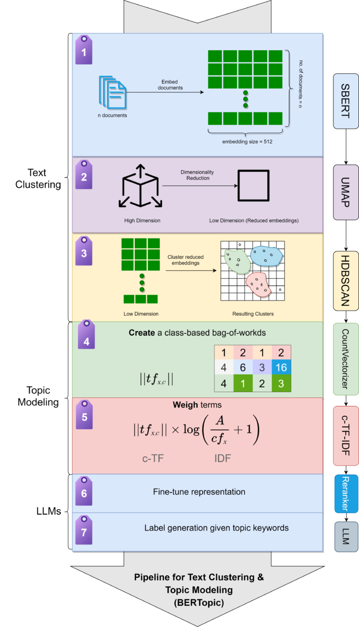
BERTopic's 6-Component Architecture
Input: Documents ↓1. Embedding Model (SBERT) → Dense vectors ↓2. Dimensionality Reduction (UMAP) → 5D vectors ↓3. Clustering (HDBSCAN) → Cluster IDs ↓4. Tokenization (CountVectorizer) → Word frequencies per cluster ↓5. Weighting (c-TF-IDF) → Important words per cluster ↓6. Representation Model (Optional) → Refined topic labels ↓Output: Topics with keywordsComponents 1-3: Same as our pipeline (Embedding → UMAP → HDBSCAN)
Components 4-6: NEW! These extract meaningful topic keywords
Component 4: CountVectorizer (Per-Cluster Tokenization)
Instead of analyzing individual documents, BERTopic concatenates all documents in a cluster and treats each cluster as one "mega-document":
from sklearn.feature_extraction.text import CountVectorizervectorizer_model = CountVectorizer( ngram_range=(1, 2), # Both single words and two-word phrases stop_words="english", # Remove common words (the, is, and, etc.) min_df=5, # Ignore words appearing in < 5 documents max_df=0.7 # Ignore words appearing in > 70% of documents)# Traditional: Each document analyzed separately# BERTopic: All documents in cluster 0 → one big document# Result: Cluster-level patterns emergeComponent 5: c-TF-IDF (The Secret Sauce!)
c-TF-IDF (class-based Term Frequency-Inverse Document Frequency) is what makes BERTopic topics so coherent.
Traditional TF-IDF:
# Finds important words in a DOCUMENT compared to corpusTF-IDF(word, document) = TF(word, doc) × log(N / df(word))c-TF-IDF:
# Finds important words in a CLUSTER compared to other clustersc-TF-IDF(word, cluster) = TF(word, cluster) × log(n_clusters / cf(word))Example in action:
Cluster 0 (Machine Learning papers):Words: learning(500×), neural(300×), model(250×), network(200×)Cluster 1 (NLP papers):Words: language(400×), text(350×), nlp(200×), processing(180×)c-TF-IDF identifies distinctive words:Cluster 0: "neural", "deep", "training", "architecture"Cluster 1: "language", "syntax", "semantic", "parsing"Without c-TF-IDF, generic words like "learning" would dominate both!Implementation:
from bertopic.vectorizers import ClassTfidfTransformerctfidf_model = ClassTfidfTransformer( reduce_frequent_words=True # Further reduce weight of very common words)Component 6: Representation Models (Optional Refinement)
Refine topics beyond c-TF-IDF keywords:
Option A: KeyBERTInspired - Extract keyphrases
from bertopic.representation import KeyBERTInspiredrepresentation_model = KeyBERTInspired()# Before (c-TF-IDF): ["neural", "network", "deep", "learning"]# After (KeyBERT): ["neural networks", "deep learning", "network architecture"]Option B: Maximal Marginal Relevance - Balance relevance and diversity
from bertopic.representation import MaximalMarginalRelevancerepresentation_model = MaximalMarginalRelevance(diversity=0.3)# Ensures keywords are relevant AND different from each other# Bad: ["learning", "learner", "learned", "learns"] (too similar)# Good: ["learning", "optimization", "regularization", "validation"] (diverse)Option C: LLM-based - Natural language labels
from bertopic.representation import OpenAIprompt = """I have a topic with keywords: [KEYWORDS]Generate a 2-5 word topic label.Only return the label."""representation_model = OpenAI( model="gpt-4", prompt=prompt)# Keywords: ["neural", "deep", "learning", "network"]# LLM Label: "Deep Neural Network Training"Installing BERTopic
# Basic installationpip install bertopic# With all optional dependenciespip install bertopic[all]# Or install components individuallypip install bertopic sentence-transformers umap-learn hdbscan scikit-learnBasic BERTopic Implementation
Simplest possible usage (3 lines):
from bertopic import BERTopic# Initialize with defaultstopic_model = BERTopic(language="english", verbose=True)# Fit and get topicstopics, probabilities = topic_model.fit_transform(documents)# View resultsprint(topic_model.get_topic_info())Output:
Topic Count Name-1 234 -1_outlier_documents 0 1247 0_machine_learning_neural_deep 1 982 1_natural_language_processing_text 2 756 2_computer_vision_image_detection 3 543 3_reinforcement_learning_agent_reward...Advanced BERTopic Configuration
Full customization of all components:
from bertopic import BERTopicfrom sentence_transformers import SentenceTransformerfrom umap import UMAPfrom hdbscan import HDBSCANfrom sklearn.feature_extraction.text import CountVectorizerfrom bertopic.vectorizers import ClassTfidfTransformerfrom bertopic.representation import KeyBERTInspired# Component 1: Embeddingembedding_model = SentenceTransformer("all-mpnet-base-v2")# Component 2: UMAPumap_model = UMAP( n_neighbors=15, n_components=5, min_dist=0.0, metric='cosine', random_state=42)# Component 3: HDBSCANhdbscan_model = HDBSCAN( min_cluster_size=15, min_samples=10, metric='euclidean', cluster_selection_method='eom', prediction_data=True)# Component 4: Vectorizervectorizer_model = CountVectorizer( ngram_range=(1, 2), stop_words="english", min_df=5, max_df=0.7)# Component 5: c-TF-IDFctfidf_model = ClassTfidfTransformer(reduce_frequent_words=True)# Component 6: Representationrepresentation_model = KeyBERTInspired()# Create BERTopic with all custom componentstopic_model = BERTopic( embedding_model=embedding_model, umap_model=umap_model, hdbscan_model=hdbscan_model, vectorizer_model=vectorizer_model, ctfidf_model=ctfidf_model, representation_model=representation_model, top_n_words=10, # Keywords per topic nr_topics="auto", # Auto topic reduction calculate_probabilities=True, # Enable soft clustering verbose=True)# Fit modeltopics, probabilities = topic_model.fit_transform(documents)print(f"✓ Discovered {len(set(topics)) - 1} topics")Working with BERTopic Results
# Get all topic informationtopic_info = topic_model.get_topic_info()print(topic_info.head())# Get specific topic keywordstopic_0_keywords = topic_model.get_topic(0)print("\nTopic 0 keywords:")for word, score in topic_0_keywords[:10]: print(f" {word:20s} {score:.4f}")# Get documents in a topictopic_0_docs = [documents[i] for i, t in enumerate(topics) if t == 0]print(f"\nTopic 0 has {len(topic_0_docs)} documents")# Search for topicssimilar_topics, similarity = topic_model.find_topics("deep learning", top_n=5)print(f"\nTopics related to 'deep learning': {similar_topics}")# Get topic distribution for new documentnew_doc = ["Latest advances in transformer models"]new_topic, new_prob = topic_model.transform(new_doc)print(f"\nNew document assigned to topic: {new_topic[0]}")5. Topic Modeling with LLMs
Topic modeling goes beyond clustering by assigning meaningful labels and descriptions to each cluster.
What is Topic Modeling?
Topic modeling identifies abstract "topics" that occur in a collection of documents. While clustering groups documents, topic modeling names and describes those groups.
Clustering: "These 100 documents are similar"
Topic Modeling: "These documents are about 'Neural Machine Translation'"
Traditional vs LLM-Based Topic Modeling
Traditional (LDA):
-
Topics are probability distributions over words
-
Output:
[("neural", 0.05), ("network", 0.04), ("deep", 0.03), ...] -
Hard to interpret
-
No semantic understanding
LLM-Based (BERTopic):
-
Topics are coherent keyword clusters
-
Output:
["neural networks", "deep learning", "training"] -
Plus optional LLM-generated label: "Deep Neural Network Training"
-
Semantically meaningful
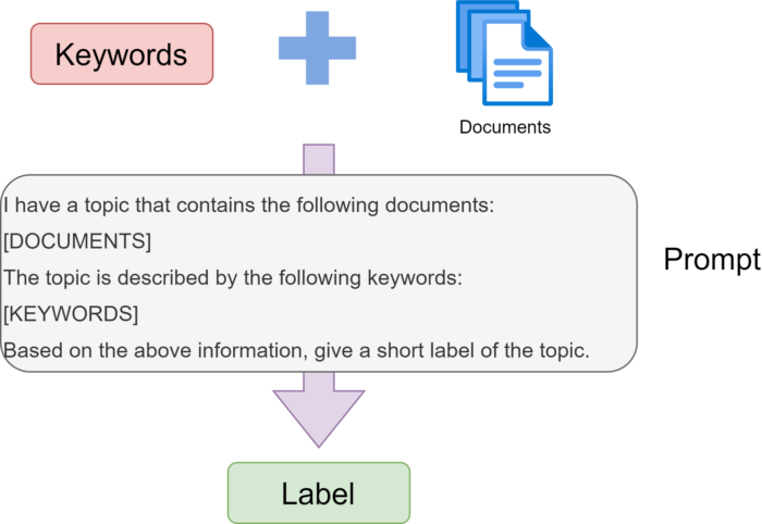
Generating Topic Labels with LLMs
The most powerful feature: using GPT-4 or Claude to create human-readable topic labels.
Method 1: BERTopic Built-in LLM Support
from bertopic.representation import OpenAIfrom bertopic import BERTopic# Configure LLM labelingprompt = """I have a topic described by these keywords: [KEYWORDS]Based on these keywords, generate a concise, descriptive topic label (2-6 words).The label should capture the main theme.Only return the label, nothing else.Keywords: [KEYWORDS]Label:"""llm_model = OpenAI( model="gpt-4", chat=True, prompt=prompt, exponential_backoff=True)# Create BERTopic with LLM labelingtopic_model = BERTopic( representation_model=llm_model, verbose=True)topics, probs = topic_model.fit_transform(documents)# View generated labelstopic_info = topic_model.get_topic_info()print(topic_info[['Topic', 'Count', 'Name']])Output:
Topic Count Name-1 234 -1_outlier_documents 0 1247 Deep Neural Network Training 1 982 Natural Language Processing 2 756 Computer Vision and Object Detection 3 543 Reinforcement Learning AlgorithmsMethod 2: Post-hoc Labeling with Claude
import anthropicdef generate_topic_label_claude(keywords, sample_docs): """Generate topic label using Claude""" client = anthropic.Anthropic(api_key="your-api-key") keywords_str = ", ".join([word for word, _ in keywords[:10]]) docs_str = "\n".join([f"• {doc[:150]}" for doc in sample_docs[:3]]) prompt = f"""<documents>Keywords that characterize this topic: {keywords_str}Sample documents from this cluster:{docs_str}</documents>Based on the keywords and sample documents, generate a concise, descriptive label (2-6 words) that captures the main theme of this topic.Respond with ONLY the label.""" message = client.messages.create( model="claude-3-5-sonnet-20241022", max_tokens=50, temperature=0.3, messages=[{"role": "user", "content": prompt}] ) return message.content[0].text.strip()# Generate labels for all topicsfor topic_id in range(len(set(topics)) - 1): keywords = topic_model.get_topic(topic_id) topic_docs = [documents[i] for i, t in enumerate(topics) if t == topic_id][:5] label = generate_topic_label_claude(keywords, topic_docs) print(f"Topic {topic_id}: {label}")6. Real-World Implementation: ArXiv Dataset Example
Let's implement a complete, production-ready clustering system using the ArXiv NLP papers dataset.
Dataset Overview
ArXiv NLP Dataset:
-
Documents: 44,949 research paper abstracts
-
Domain: Computation and Language (cs.CL)
-
Years: 1991-2024
-
Source: Hugging Face (
maartengr/arxiv_nlp)
Complete Implementation
"""ArXiv NLP Paper ClusteringComplete pipeline from data loading to visualization"""# Step 1: Load Datafrom datasets import load_datasetprint("Loading ArXiv NLP dataset...")dataset = load_dataset("maartengr/arxiv_nlp")["train"]abstracts = dataset["Abstracts"]titles = dataset["Titles"]print(f"✓ Loaded {len(abstracts)} papers")# Step 2: Generate Embeddingsfrom sentence_transformers import SentenceTransformerprint("\n[1/3] Generating embeddings...")embedding_model = SentenceTransformer("all-mpnet-base-v2")embeddings = embedding_model.encode( abstracts, batch_size=32, show_progress_bar=True, normalize_embeddings=True)print(f"✓ Generated {embeddings.shape} embeddings")# Step 3: Create BERTopic Modelfrom bertopic import BERTopicfrom umap import UMAPfrom hdbscan import HDBSCANfrom sklearn.feature_extraction.text import CountVectorizerfrom bertopic.vectorizers import ClassTfidfTransformerprint("\n[2/3] Configuring BERTopic...")umap_model = UMAP( n_neighbors=15, n_components=5, min_dist=0.0, metric='cosine', random_state=42)hdbscan_model = HDBSCAN( min_cluster_size=15, min_samples=10, metric='euclidean', cluster_selection_method='eom')vectorizer_model = CountVectorizer( ngram_range=(1, 2), stop_words="english", min_df=5)ctfidf_model = ClassTfidfTransformer(reduce_frequent_words=True)topic_model = BERTopic( embedding_model=embedding_model, umap_model=umap_model, hdbscan_model=hdbscan_model, vectorizer_model=vectorizer_model, ctfidf_model=ctfidf_model, top_n_words=10, verbose=True)# Step 4: Fit Modelprint("\n[3/3] Clustering and extracting topics...")topics, probabilities = topic_model.fit_transform(abstracts, embeddings)n_topics = len(set(topics)) - 1n_outliers = list(topics).count(-1)print(f"\n{'='*60}")print("RESULTS")print(f"{'='*60}")print(f"✓ Discovered {n_topics} topics")print(f"✓ Outliers: {n_outliers} ({n_outliers/len(topics)*100:.1f}%)")# Step 5: Inspect Topicstopic_info = topic_model.get_topic_info()print(f"\nTop 10 Topics:")print(topic_info.head(11)[['Topic', 'Count', 'Name']])# Step 6: Detailed Topic Inspectionprint(f"\n{'='*60}")print("TOPIC DETAILS")print(f"{'='*60}")for i in range(min(5, n_topics)): topic_id = topic_info.iloc[i+1]['Topic'] # Skip -1 topic_size = topic_info.iloc[i+1]['Count'] print(f"\nTOPIC {topic_id} ({topic_size} papers)") print("-" * 60) # Keywords topic_words = topic_model.get_topic(topic_id) print("Keywords:") for word, score in topic_words[:8]: print(f" {word:25s} {score:.4f}") # Sample papers topic_papers = [(i, titles[i]) for i, t in enumerate(topics) if t == topic_id] print(f"\nSample papers:") for j, (idx, title) in enumerate(topic_papers[:3]): print(f" {j+1}. {title}")# Step 7: Save Modelprint(f"\n{'='*60}")print("SAVING")print(f"{'='*60}")topic_model.save("arxiv_bertopic_model")print("✓ Model saved to arxiv_bertopic_model/")# Step 8: Visualizationsprint("\nGenerating visualizations...")# Topic mapfig1 = topic_model.visualize_topics()fig1.write_html("arxiv_topics_map.html")print("✓ Saved: arxiv_topics_map.html")# Bar chartfig2 = topic_model.visualize_barchart(top_n_topics=20, n_words=8)fig2.write_html("arxiv_barchart.html")print("✓ Saved: arxiv_barchart.html")# Hierarchyfig3 = topic_model.visualize_hierarchy()fig3.write_html("arxiv_hierarchy.html")print("✓ Saved: arxiv_hierarchy.html")print(f"\n{'='*60}")print("✓ COMPLETE!")print(f"{'='*60}")Expected Output:
Loading ArXiv NLP dataset...✓ Loaded 44,949 papers[1/3] Generating embeddings...100%|██████████| 1405/1405 [08:32<00:00, 2.74it/s]✓ Generated (44949, 768) embeddings[2/3] Configuring BERTopic...[3/3] Clustering and extracting topics...============================================================RESULTS============================================================✓ Discovered 127 topics✓ Outliers: 2,341 (5.2%)Top 10 Topics:Topic Count Name-1 2341 -1_outliers 0 3456 0_neural_machine_translation 1 2234 1_question_answering_reading 2 1876 2_sentiment_analysis_opinion 3 1654 3_named_entity_recognition 4 1432 4_speech_recognition_acoustic...============================================================TOPIC DETAILS============================================================TOPIC 0 (3456 papers)------------------------------------------------------------Keywords: neural 0.0234 machine 0.0198 translation 0.0187 nmt 0.0156 encoder 0.0142 decoder 0.0138 attention 0.0121 transformer 0.0109Sample papers: 1. Attention Is All You Need 2. Neural Machine Translation by Jointly Learning to Align and Translate 3. Effective Approaches to Attention-based Neural Machine Translation[... continues for topics 1-4 ...]============================================================SAVING============================================================✓ Model saved to arxiv_bertopic_model/Generating visualizations...✓ Saved: arxiv_topics_map.html✓ Saved: arxiv_barchart.html✓ Saved: arxiv_hierarchy.html============================================================✓ COMPLETE!============================================================Results Analysis
# Calculate quality metricsfrom sklearn.metrics import silhouette_scoremask = topics != -1silhouette = silhouette_score( embeddings[mask][:10000], # Sample for speed topics[mask][:10000], metric='cosine')print(f"Clustering Quality:")print(f" • Silhouette Score: {silhouette:.4f}")print(f" {'Excellent' if silhouette > 0.7 else 'Good' if silhouette > 0.5 else 'Moderate'}")# Find most interesting topicsimport pandas as pdtopic_sizes = pd.Series(topics[mask]).value_counts()print(f"\n • Largest cluster: {topic_sizes.max()} papers")print(f" • Smallest cluster: {topic_sizes.min()} papers")print(f" • Average size: {topic_sizes.mean():.1f} papers")# Niche but significant topicsniche_topics = topic_info[ (topic_info['Count'] > 50) & (topic_info['Count'] < 200)]print(f"\nNiche Topics (50-200 papers):")for idx, row in niche_topics.head(5).iterrows(): if row['Topic'] == -1: continue print(f" • Topic {row['Topic']}: {row['Name']} ({row['Count']} papers)")8. Production Deployment Best Practices
Model Selection Guidelines
Decision Matrix:
| Dataset Size | Speed Priority | Quality Priority | Recommended Setup |
|---|---|---|---|
| < 1K docs | High | Medium | MiniLM + UMAP + K-Means |
| 1K-10K | Medium | High | mpnet + UMAP + HDBSCAN |
| 10K-100K | High | High | mpnet + UMAP + HDBSCAN + batching |
| 100K+ | High | Medium | MiniLM + PCA + MiniBatchKMeans |
Performance Optimization
# 1. Use GPU accelerationembedding_model = SentenceTransformer("all-mpnet-base-v2", device="cuda")# 2. Enable mixed precisionembeddings = embedding_model.encode( documents, batch_size=64, convert_to_numpy=True, show_progress_bar=True, normalize_embeddings=True # Faster cosine similarity)# 3. Cache embeddingsimport joblib# Savejoblib.dump(embeddings, "embeddings.pkl")# Loadembeddings = joblib.load("embeddings.pkl")# 4. Use approximate nearest neighbors for large datasetsfrom annoy import AnnoyIndexdef build_annoy_index(embeddings, n_trees=10): dimension = embeddings.shape[1] index = AnnoyIndex(dimension, 'angular') for i, emb in enumerate(embeddings): index.add_item(i, emb) index.build(n_trees) return indexMonitoring and Evaluation
import loggingfrom datetime import datetimeclass ClusteringMonitor: """Monitor clustering performance in production""" def __init__(self, log_file="clustering_metrics.log"): logging.basicConfig( filename=log_file, level=logging.INFO, format='%(asctime)s - %(message)s' ) self.logger = logging.getLogger(__name__) def log_clustering_run(self, n_docs, n_clusters, n_outliers, silhouette, runtime): """Log clustering metrics""" metrics = { 'timestamp': datetime.now().isoformat(), 'n_documents': n_docs, 'n_clusters': n_clusters, 'n_outliers': n_outliers, 'outlier_pct': n_outliers / n_docs * 100, 'silhouette_score': silhouette, 'runtime_seconds': runtime } self.logger.info(f"Clustering run: {metrics}") # Alert if quality drops if silhouette < 0.3: self.logger.warning(f"Low silhouette score: {silhouette}") if n_outliers / n_docs > 0.2: self.logger.warning(f"High outlier rate: {n_outliers/n_docs*100:.1f}%") def log_topic_update(self, topic_id, old_keywords, new_keywords): """Log topic changes""" added = set(new_keywords) - set(old_keywords) removed = set(old_keywords) - set(new_keywords) if added or removed: self.logger.info( f"Topic {topic_id} changed - Added: {added}, Removed: {removed}" )# Usagemonitor = ClusteringMonitor()import timestart = time.time()# Run clusteringtopic_model = BERTopic()topics, probs = topic_model.fit_transform(documents)runtime = time.time() - start# Calculate metricsfrom sklearn.metrics import silhouette_scoren_outliers = list(topics).count(-1)mask = topics != -1silhouette = silhouette_score(embeddings[mask], topics[mask], metric='cosine')# Logmonitor.log_clustering_run( n_docs=len(documents), n_clusters=len(set(topics)) - 1, n_outliers=n_outliers, silhouette=silhouette, runtime=runtime)9. Common Challenges and Solutions
Challenge 1: Too Many Small Clusters
Problem: HDBSCAN creates 100+ tiny clusters instead of meaningful groups
Symptoms:
-
Many clusters with 10-20 documents
-
Fragmented topics
-
Hard to interpret
Solutions:
# Solution 1: Increase min_cluster_sizehdbscan_model = HDBSCAN( min_cluster_size=50, # Increase from 15 min_samples=10)# Solution 2: Use topic reduction in BERTopictopic_model = BERTopic( hdbscan_model=hdbscan_model, nr_topics=20 # Reduce to 20 topics)# Solution 3: Post-hoc mergingtopic_model.reduce_topics(documents, topics, nr_topics=20)# Solution 4: Adjust UMAP parameters for less granularityumap_model = UMAP( n_neighbors=30, # Increase (was 15) n_components=5, min_dist=0.1 # Increase (was 0.0))Challenge 2: Poor Topic Coherence
Problem: Topics contain unrelated or nonsensical keywords
Solutions:
# Solution 1: Better preprocessingdef preprocess_text(text): # Remove URLs text = re.sub(r'http\S+', '', text) # Remove emails text = re.sub(r'\S+@\S+', '', text) # Remove numbers text = re.sub(r'\d+', '', text) # Remove extra whitespace text = ' '.join(text.split()) return text.lower()documents_clean = [preprocess_text(doc) for doc in documents]# Solution 2: Better stopword handlingvectorizer_model = CountVectorizer( ngram_range=(1, 2), stop_words="english", min_df=10, # Increase (ignore very rare words) max_df=0.5 # Decrease (ignore very common words))# Solution 3: Use representation modelsfrom bertopic.representation import KeyBERTInspired, MaximalMarginalRelevancerepresentation_models = [ KeyBERTInspired(), MaximalMarginalRelevance(diversity=0.3)]topic_model = BERTopic( representation_model=representation_models)# Solution 4: Manual topic refinement# Merge similar topicstopics_to_merge = [[1, 5], [3, 7], [9, 12]]topic_model.merge_topics(documents, topics, topics_to_merge)Challenge 3: High Outlier Rate (>20%)
Problem: Too many documents classified as outliers (-1 cluster)
Solutions:
# Solution 1: Reduce min_sampleshdbscan_model = HDBSCAN( min_cluster_size=15, min_samples=5, # Decrease (was 10) metric='euclidean')# Solution 2: Try different distance metrichdbscan_model = HDBSCAN( min_cluster_size=15, metric='manhattan', # Try instead of euclidean cluster_selection_method='eom')# Solution 3: Reduce dimensionality less aggressivelyumap_model = UMAP( n_neighbors=15, n_components=10, # Increase (was 5) min_dist=0.0)# Solution 4: Assign outliers to nearest clusterdef assign_outliers_to_nearest_cluster(embeddings, clusters): from scipy.spatial.distance import cdist outlier_mask = clusters == -1 outlier_indices = np.where(outlier_mask)[0] # Get cluster centroids cluster_ids = set(clusters) - {-1} centroids = {} for cluster_id in cluster_ids: cluster_points = embeddings[clusters == cluster_id] centroids[cluster_id] = cluster_points.mean(axis=0) # Assign each outlier to nearest centroid for idx in outlier_indices: distances = { cid: np.linalg.norm(embeddings[idx] - centroid) for cid, centroid in centroids.items() } nearest_cluster = min(distances, key=distances.get) clusters[idx] = nearest_cluster return clusters# Applyclusters_fixed = assign_outliers_to_nearest_cluster(embeddings, clusters.copy())Challenge 4: Slow Performance
Problem: Clustering takes too long on large datasets
Solutions:
# Solution 1: Use smaller embedding modelembedding_model = SentenceTransformer("all-MiniLM-L6-v2") # Fast, 80MB# Solution 2: Sample large datasetssample_size = 10000sample_indices = np.random.choice(len(documents), sample_size, replace=False)sample_docs = [documents[i] for i in sample_indices]# Cluster sampletopic_model = BERTopic()topics, probs = topic_model.fit_transform(sample_docs)# Predict on full datasetall_topics, all_probs = topic_model.transform(documents)# Solution 3: Use approximate UMAPumap_model = UMAP( n_neighbors=15, n_components=5, metric='cosine', low_memory=True, # Use less memory, slightly slower random_state=42)# Solution 4: Parallel processingfrom multiprocessing import Pooldef process_batch(batch): return embedding_model.encode(batch)# Split into batchesbatch_size = 1000batches = [documents[i:i+batch_size] for i in range(0, len(documents), batch_size)]# Process in parallelwith Pool(processes=4) as pool: batch_embeddings = pool.map(process_batch, batches)embeddings = np.vstack(batch_embeddings)10. Comparison: BERTopic vs Alternatives
vs Traditional LDA
| Aspect | LDA | BERTopic |
|---|---|---|
| Input | Bag-of-words | Embeddings |
| Context | ❌ None | ✅ Contextual |
| # Topics | ⚠️ Must specify | ✅ Auto-discovers |
| Outliers | ❌ Forces assignment | ✅ Explicit -1 cluster |
| Short text | ❌ Poor | ✅ Excellent |
| Speed | ✅ Fast | ⚠️ Slower |
| Interpretability | ⚠️ Probability distributions | ✅ Clear keywords |
| Reproducibility | ⚠️ Varies | ✅ Deterministic (with seed) |
vs Top2Vec
| Aspect | Top2Vec | BERTopic |
|---|---|---|
| Architecture | Doc2Vec + UMAP + HDBSCAN | SBERT + UMAP + HDBSCAN |
| Modularity | ❌ Fixed pipeline | ✅ Fully modular |
| Customization | ⚠️ Limited | ✅ Extensive |
| Topic refinement | ❌ Basic | ✅ Multiple representation models |
| Online learning | ✅ Yes | ✅ Yes |
| Hierarchical | ❌ No | ✅ Yes |
| Dynamic modeling | ❌ No | ✅ Yes |
vs CTM (Contextualized Topic Models)
| Aspect | CTM | BERTopic |
|---|---|---|
| Base model | BERT + Neural Variational | SBERT + HDBSCAN |
| Complexity | ⚠️ High | ✅ Medium |
| Training time | ⚠️ Slow | ✅ Fast |
| Stability | ⚠️ Requires tuning | ✅ Stable defaults |
| Zero-shot | ❌ Needs training | ✅ Immediate |
| Documentation | ⚠️ Limited | ✅ Extensive |
| Community | ⚠️ Small | ✅ Large |
When to Use What
Use LDA when:
-
You need very fast processing
-
Working with large, clean corpora
-
Interpretable probability distributions are important
-
Limited computational resources
Use Top2Vec when:
-
You want Doc2Vec embeddings specifically
-
Simpler API preferred
-
Don't need customization
Use CTM when:
-
Academic research context
-
Need probabilistic framework
-
Have computational resources for training
Use BERTopic when:
-
Need production-ready solution ✅
-
Want modular, customizable pipeline ✅
-
Working with diverse text types ✅
-
Need hierarchical topics ✅
-
Want dynamic/online modeling ✅
-
Require extensive documentation ✅
11. Tools and Resources
Python Libraries
Core Libraries:
# Essentialpip install bertopic sentence-transformers umap-learn hdbscan# Visualizationpip install plotly datamapplot# Optional enhancementspip install spacypython -m spacy download en_core_web_sm# For LLM labelingpip install openai anthropicAlternative Libraries:
# Traditional topic modelingpip install gensim # For LDApip install scikit-learn # For NMF, LSA# Other embedding modelspip install transformers torch# Approximate nearest neighborspip install annoy faiss-cpuEmbedding Models
General Purpose (Recommended):
-
all-MiniLM-L6-v2- Fast, 384-dim, 80MB -
all-mpnet-base-v2- High quality, 768-dim, 420MB -
stella-en-400M-v5- State-of-the-art, 1024-dim, 1.6GB
Domain-Specific:
-
allenai/specter- Scientific papers -
biobert-base-cased- Biomedical text -
finbert- Financial documents -
legal-bert-base-uncased- Legal documents
Multilingual:
-
paraphrase-multilingual-MiniLM-L12-v2- 50+ languages -
distiluse-base-multilingual-cased-v2- Fast multilingual
Find more: MTEB Leaderboard
Datasets for Practice
- 20 Newsgroups - Classic text classification
from sklearn.datasets import fetch_20newsgroupsdocs = fetch_20newsgroups(subset='all')['data']- ArXiv Papers - Academic abstracts
from datasets import load_datasetdataset = load_dataset("maartengr/arxiv_nlp")- BBC News - News articles
# Download from: http://mlg.ucd.ie/datasets/bbc.html- Amazon Reviews - Product reviews
from datasets import load_datasetdataset = load_dataset("amazon_polarity")- Twitter Sentiment - Short texts
from datasets import load_datasetdataset = load_dataset("tweet_eval", "sentiment")Documentation & Tutorials
Official Documentation:
Tutorials:
Books:
- Hands-On Large Language Models by Jay Alammar & Maarten Grootendorst
Research Papers:
12. Frequently Asked Questions
Q1: What's the difference between text clustering and topic modeling?
A: Text clustering groups similar documents together based on semantic meaning, while topic modeling labels and describes those groups with keywords or phrases.
Think of it this way:
-
Clustering: "These 100 documents are similar" (grouping)
-
Topic modeling: "These documents are about 'neural networks and deep learning'" (labeling)
In practice, topic modeling often follows clustering. BERTopic combines both: it clusters documents (Stage 1-3) then extracts topics (Stage 4-6).
Q2: Why use BERTopic instead of traditional LDA for topic modeling?
A: BERTopic offers several advantages:
-
Contextual understanding: Uses BERT embeddings that understand "bank" (river) vs "bank" (financial)
-
No K specification: Discovers optimal number of topics automatically
-
Better outlier handling: HDBSCAN explicitly identifies outliers (-1 cluster)
-
Short text performance: Works well with tweets, reviews (LDA struggles)
-
Modularity: Swap components (embedding model, clustering algorithm, etc.)
-
Topic coherence: Generally produces more interpretable topics
When to use LDA:
-
Very large datasets (millions of documents)
-
Extremely limited compute resources
-
Need probabilistic topic distributions
-
Academic research requiring traditional methods
Q3: What does the -1 cluster in HDBSCAN represent?
A: The -1 cluster represents outliers - documents that don't fit well into any cluster. These are data points too far from dense regions to be assigned to a cluster.
Common outlier types:
-
🔍 Legitimate edge cases (rare, unique topics)
-
🗑️ Noise, spam, or low-quality text
-
📝 Multi-topic documents blending themes
-
⚠️ Very short documents lacking context
Handling strategies:
-
Keep separate: Review manually, may contain insights
-
Assign to nearest: Use distance to cluster centroids
-
Adjust parameters: Reduce
min_samplesto be less strict -
Accept as normal: 5-10% outliers is typical and healthy
Q4: Which embedding model should I use for text clustering?
A: Choose based on your priorities:
Speed priority:
-
all-MiniLM-L6-v2(384-dim, 80MB, ~1000 docs/sec) -
Best for: Prototyping, large datasets, real-time systems
Quality priority:
-
all-mpnet-base-v2(768-dim, 420MB, ~400 docs/sec) -
Best for: Production systems, critical applications
Bleeding edge:
-
stella-en-400M-v5(1024-dim, 1.6GB, ~200 docs/sec) -
Best for: Research, maximum accuracy
Domain-specific:
-
Scientific papers:
allenai/specter -
Medical:
biobert-base-cased -
Financial:
finbert -
Legal:
legal-bert-base-uncased
Always test on a sample of your data! Embeddings that work well for news articles may not be optimal for tweets.
Q5: Can BERTopic handle documents in multiple languages?
A: Yes! Use a multilingual embedding model:
from sentence_transformers import SentenceTransformer# Supports 50+ languagesmultilingual_model = SentenceTransformer( "paraphrase-multilingual-MiniLM-L12-v2")topic_model = BERTopic( embedding_model=multilingual_model, language="multilingual")# Works with mixed-language documentsdocs = [ "Machine learning is powerful", # English "El aprendizaje automático es poderoso", # Spanish "機械学習は強力です" # Japanese]topics, probs = topic_model.fit_transform(docs)Important notes:
-
All documents embedded in same semantic space
-
Similar concepts cluster together regardless of language
-
Topic keywords may include multiple languages
-
For best single-language results, use language-specific models
Q6: How do I choose the right number of clusters?
A: Great news - you don't have to! HDBSCAN automatically discovers the optimal number based on data density.
What HDBSCAN does:
-
Finds dense regions in embedding space
-
Groups documents in dense regions into clusters
-
Marks isolated documents as outliers (-1)
-
Number of clusters emerges naturally from data
If you want control:
# More clusters (smaller groups)hdbscan_model = HDBSCAN( min_cluster_size=10, # Smaller minimum min_samples=5)# Fewer clusters (larger groups)hdbscan_model = HDBSCAN( min_cluster_size=50, # Larger minimum min_samples=10)# Or reduce topics post-hoctopic_model.reduce_topics(documents, topics, nr_topics=20)Rule of thumb:
-
1,000 docs → expect 10-30 clusters
-
10,000 docs → expect 50-150 clusters
-
100,000 docs → expect 100-300 clusters
Q7: How does c-TF-IDF differ from regular TF-IDF?
A: The key difference is the level of analysis:
Traditional TF-IDF:
-
Analyzes individual documents
-
Finds important words per document
-
Formula: TF(word, doc) × IDF(word, corpus)
c-TF-IDF (class-based):
-
Analyzes clusters (treats each cluster as one "mega-document")
-
Finds important words per cluster
-
Formula: TF(word, cluster) × IDF(word, all_clusters)
Example:
# Cluster 0: ML papers# Contains words: learning (500×), neural (300×), model (250×)# Cluster 1: NLP papers # Contains words: language (400×), text (350×), nlp (200×)# c-TF-IDF identifies:# Cluster 0 distinctive words: "neural", "deep", "network"# Cluster 1 distinctive words: "language", "syntax", "semantic"# Regular TF-IDF would miss cluster-level patterns!# Cluster 0: ML papers# Contains words: learning (500×), neural (300×), model (250×)# Cluster 1: NLP papers # Contains words: language (400×), text (350×), nlp (200×)# c-TF-IDF identifies:# Cluster 0 distinctive words: "neural", "deep", "network"# Cluster 1 distinctive words: "language", "syntax", "semantic"# Regular TF-IDF would miss cluster-level patterns!Why it matters: c-TF-IDF produces more coherent, interpretable topics because it considers the cluster context.
Q8: Is BERTopic suitable for short texts like tweets?
A: Yes! BERTopic handles short texts much better than traditional methods like LDA.
Why it works:
-
Embeddings capture semantics even from few words
-
Contextual understanding helps with abbreviations
-
Handles informal language, emojis, hashtags
Best practices for short texts:
# 1. Use smaller min_cluster_sizehdbscan_model = HDBSCAN( min_cluster_size=10, # Lower for short texts min_samples=5)# 2. Keep bigramsvectorizer_model = CountVectorizer( ngram_range=(1, 2), # Unigrams and bigrams stop_words="english")# 3. Consider shorter keywordstopic_model = BERTopic( top_n_words=5, # Fewer keywords for short texts hdbscan_model=hdbscan_model, vectorizer_model=vectorizer_model)Minimum text length: Generally works well with 5-10 words. Below that, consider:
-
Combining related short texts
-
Using bigrams/trigrams
-
Specialized short-text embeddings
Q9: How do I handle imbalanced datasets where some topics dominate?
A: Several strategies:
# Strategy 1: Normalize cluster sizes with nr_topicstopic_model = BERTopic(nr_topics=50) # Force 50 equal topics# Strategy 2: Adjust min_cluster_size dynamically# Smaller clusters for minority topicshdbscan_model = HDBSCAN( min_cluster_size=15, cluster_selection_epsilon=0.5 # Merge similar clusters)# Strategy 3: Oversample minority topicsfrom sklearn.utils import resample# Identify small clusterscluster_counts = pd.Series(topics).value_counts()small_clusters = cluster_counts[cluster_counts < 100].index# Oversample documents from small clustersoversampled_docs = []oversampled_topics = []for cluster_id in small_clusters: cluster_docs = [documents[i] for i, t in enumerate(topics) if t == cluster_id] cluster_topics = [topics[i] for i, t in enumerate(topics) if t == cluster_id] # Oversample to 100 documents resampled = resample( cluster_docs, n_samples=100, replace=True ) oversampled_docs.extend(resampled)# Retrain with balanced datatopic_model.update_topics(oversampled_docs, oversampled_topics)Q10: Can I update topics with new documents without retraining?
A: Yes! BERTopic supports incremental updates:
# Initial trainingtopic_model = BERTopic()topics, probs = topic_model.fit_transform(initial_documents)# New documents arrivenew_documents = ["Latest AI research paper", "Novel NLP technique", ...]# Option 1: Assign to existing topics (fast)new_topics, new_probs = topic_model.transform(new_documents)# Option 2: Update model with new documents (slower, more accurate)all_documents = initial_documents + new_documentsall_topics = list(topics) + list(new_topics)topic_model.update_topics( docs=all_documents, topics=all_topics, vectorizer_model=updated_vectorizer)# Topics now reflect both old and new documentsWhen to use each:
-
transform(): Daily/weekly updates, streaming data
-
update_topics(): Monthly/quarterly, significant new content
13. Conclusion
Text clustering with LLMs represents a paradigm shift from keyword-matching to semantic understanding. By combining powerful embedding models (SBERT), effective dimensionality reduction (UMAP), and density-based clustering (HDBSCAN), we can automatically discover meaningful patterns in unstructured text at scale.
Key Takeaways
✅ LLM embeddings capture semantics that traditional bag-of-words methods miss
✅ BERTopic provides a modular framework that's both powerful and customizable
✅ Three-stage pipeline (embed → reduce → cluster) is the foundation
✅ c-TF-IDF extracts distinctive keywords by analyzing clusters, not documents
✅ Production deployment requires careful attention to scalability and monitoring
✅ No one-size-fits-all solution - tune parameters for your specific use case
When to Use Text Clustering
Perfect for:
-
Organizing large document collections (research papers, support tickets)
-
Discovering emerging themes (social media, news monitoring)
-
Data exploration before building classifiers
-
Identifying outliers and data quality issues
-
Creating semantic navigation systems
Not ideal for:
-
Real-time classification (use trained classifiers instead)
-
When you need specific predefined categories (use classification)
-
Tiny datasets (<100 documents)
-
When interpretability isn't important
Implementation Checklist
Phase 1: Prototype (1-2 days)
-
[ ] Install BERTopic and dependencies
-
[ ] Load and explore your dataset
-
[ ] Run basic clustering with defaults
-
[ ] Inspect top 10 topics manually
-
[ ] Assess if approach is viable
Phase 2: Optimization (3-5 days)
-
[ ] Test different embedding models
-
[ ] Tune UMAP parameters (n_neighbors, n_components)
-
[ ] Tune HDBSCAN parameters (min_cluster_size, min_samples)
-
[ ] Experiment with representation models
-
[ ] Calculate quality metrics (silhouette, coherence)
Phase 3: Production (1-2 weeks)
-
[ ] Implement batch processing for large datasets
-
[ ] Add error handling and retries
-
[ ] Set up monitoring and logging
-
[ ] Create visualization dashboards
-
[ ] Document model parameters and decisions
-
[ ] Plan update strategy for new documents
Next Steps
Immediate actions:
-
Download the code
-
Try clustering on your own dataset
-
Share results and questions in comments
Get Help
Questions? Drop a comment below - I respond within 24 hours
Found value? Share this guide with your team
References
-
Grootendorst, M. (2022). BERTopic: Neural topic modeling with a class-based TF-IDF procedure. arXiv preprint arXiv:2203.05794.
-
Reimers, N., & Gurevych, I. (2019). Sentence-BERT: Sentence Embeddings using Siamese BERT-Networks. EMNLP 2019.
-
McInnes, L., Healy, J., & Astels, S. (2017). hdbscan: Hierarchical density based clustering. Journal of Open Source Software, 2(11), 205.
-
McInnes, L., Healy, J., & Melville, J. (2018). UMAP: Uniform Manifold Approximation and Projection for Dimension Reduction. arXiv preprint arXiv:1802.03426.
-
Devlin, J., Chang, M. W., Lee, K., & Toutanova, K. (2018). BERT: Pre-training of Deep Bidirectional Transformers for Language Understanding. NAACL 2019.
© 2025 Ranjan Kumar. All rights reserved.
Related Articles
Natural Language Processing Nlp
- Hands-on Tutorial on Making an Audio Bot using LLM, and RAG
- How Google's SynthID Actually Works: A Visual Breakdown
- Introducing My New Book: The ChatML (Chat Markup Language) Handbook
Follow for more technical deep dives on AI/ML systems, production engineering, and building real-world applications:


